Honestly speaking, assumptions are a main part of physics. These are the reasons why some physical calculations work while others don’t. Why some rockets fly and others don’t. It’s not like those scientists can’t calculate ,but, since physics is an integral part of the calculations and it is based on so many assumptions (note these are simplifications and not inaccuracies).
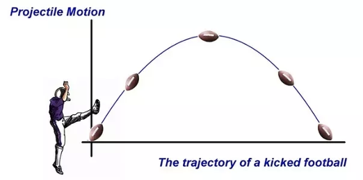
Projectile motion, one of physics’ simplest concepts, often relies on assumptions that streamline its complexity. But when real-world factors—like wind, Earth’s rotation, and drag—are added, the elegance of simple equations breaks down, revealing the true depth of this phenomenon. But, worry not, I spent countless nights and days studying Projectile Motion and the assumptions we make. I could not find any other research paper or journal on the equation of projectile motion without assumption, hence, I fear I may be the first one to try this.
The assumptions of projectile motion in simple mechanics;
- Negligible Air Resistance
- No effect of Earth’s rotation
- No effect of Earth’s revolution around the sun
- Constant acceleration due to gravity around the surface of the earth
- Simplification of surface of object as 1 m^2
- And finally no effect of wind.
Let’s deal with them individually and then we will combine them;
Air Resistance
Air resistance can be simply understood by using linear air drag or simply linear drag. The surface of the earth usually applies somewhere between linear and quadratic drag not one of them, as both (linear and quadratic drag) have no place other than our imaginations. We can accommodate this air drag later, but for now, we will follow a simple linear drag. It would be adjusted later when we start with wind effects.
Hence, the drag term can be written as:
Yeah, this is the equation, I don’t really want to bore you with the derivation over here. But will give you a glimpse.
Newton’s Second Law of Motion: We start with Newton’s second law of motion, which states that the net force on an object is equal to the mass of the object times its acceleration:
Drag Force Proportional to Velocity: In the case of linear drag, the force due to air resistance is proportional to the velocity of the object:
The negative sign indicates that the drag force opposes the motion (i.e., acts in the opposite direction to the velocity vector).
Including Gravitational Force: If we assume the object is moving in a gravitational field, the total net force on the object will be the sum of the gravitational force and the drag force. The gravitational force is given by:
So the total force becomes:
Substitute into Newton’s Second Law: Now, substitute this total force into Newton’s second law:
Solve for Acceleration: Divide through by the mass mmm to get the equation in terms of acceleration:
This is the equation of motion for an object experiencing both gravity and linear air resistance. The term  represents the acceleration due to air drag, while
  represents the acceleration due to gravity.
Why did you choose to focus on linear drag rather than quadratic drag, which might better represent real-world conditions?
Both linear drag and quadratic drag provide almost identical results at low speeds (such as 10^{-8} times the speed of light). At these speeds, the differences between the two drag models are negligible, making linear drag a suitable approximation. However, as velocities increase, particularly around 10^{-4} times the speed of light (about 30 km/s), these differences become significant, and quadratic drag tends to offer a more accurate model.
In this simulation, I focused on linear drag for simplicity and computational efficiency. While quadratic drag can offer a more precise representation at higher speeds, linear drag allows us to capture the core dynamics of projectile motion without overwhelming complexity. It also gives a good approximation for everyday projectiles (like thrown objects or sports balls) where the velocity remains far below the range where quadratic drag becomes crucial.
Coriolis Force (Effect due to rotation of Earth)
Having addressed air resistance, we now turn to the Coriolis force, a subtle yet significant player in the motion of projectiles. Though Coriolis Force is hard to differentiate from Euler Force or Centripetal Force, some simplifications (though these are not based on numerical values) but rather on theory.
Coriolis Force can be defined numerically as:
Again, I won’t go much in derivation as this is a well-known formula and one can easily find it on trustable sources like, Coriolis force – Wikipedia.
Is the Coriolis effect significant for everyday projectiles, or does it only matter in extreme cases like long-range missiles or artillery?
Coriolis effects are usually related to long distances, and don’t have a large effect on small-scale projectiles. But, they still act and they have a significant impact on small-scale projectiles also, especially on the downward path of the projectile after it reaches its peak. It slows its horizontal velocity and thus makes it fall sooner. In our calculation, the difference was about 9m.
It affects the horizontal velocity more significantly during the descent, where the rotation of the Earth becomes more noticeable as the projectile slows.
Centripetal Force
Again, this can be easily defined by formulas, usually, we use this formula,
This formula is very well known and used in many applications. Centripetal force would be applied, and hence would disrupt the acceleration of the projectile.
How does the inclusion of centrifugal force affect the overall trajectory compared to traditional projectile motion without it?
The inclusion of centrifugal force affects the overall trajectory only slightly compared to traditional projectile motion without it. Centrifugal force arises due to the Earth’s rotation and acts outward from the center of rotation, opposing gravitational pull to a small extent. In this case, the acceleration due to centrifugal force is about 10^{−3} m/(s^2), which is negligible compared to gravity (around 9.81 m/s2).
For most practical situations, such as sports or short-range projectiles, this effect is minimal and can be ignored. However, for very long-range projectiles (e.g., missiles or artillery), or at higher altitudes, the small change in trajectory due to centrifugal force could become more relevant. Hence, its inclusion was necessary.
Variable Gravitational Effect
Though this effect can be measured, but the actual working of this effect is not based on any formula. Though scientists have offered various formulas like:
But, experiments showed these don’t actually hold true and acceleration due to gravity follows an unknown pattern which doesn’t follow any formula. Hence, for simplicity sake, we may define it as
or g as a function of the height of the object, as no working formula is present.
For the code however, we use the formula which is derived from Newton’s Third Law. It’s important to note that this formula is a simplification. It doesn’t account for factors like latitudinal and longitudinal variations in Earth’s gravitational field. Additionally, experimental data presented at the Physics Conference in 1968 revealed a far more intricate variation in gravity than a simple quadratic curve suggests. However, for the purposes of this simulation, we’ve chosen to use this simplified model to demonstrate the general impact of a changing gravitational force on projectile motion. And Variable Acc. due to gravity doesn’t have an significant impact on the projectile until it reaches over 10^4m in the air. Then only its effects are more determinable.
Wind Effects
To include the effect of wind, the equation needs to account for the relative velocity between the projectile and the wind. Let’s denote the wind velocity as  . The drag force should then be based on the relative velocity
The drag term in the equation would be modified to:
Final Equation
Where:
- c is the drag coefficient.
- m is the mass of the projectile.
- All other variables have been defined earlier.
How do you check if it is true?
Equations such as these can be solved by either using double-integration or by using python code. Since, doing all this by hand is a hefty task and can lead to errors. We use computer code, usually Python. One such code for this with sample values is:
import numpy as np
from scipy.integrate import solve_ivp
import matplotlib.pyplot as plt

# Constants
g = 9.81  # Acceleration due to gravity (m/s^2)
c = 0.07  # Drag coefficient (kg/s)
m = 1   # Mass of the object (kg)
Omega = 7.2921e-5  # Angular velocity of the Earth (rad/s)

# Wind velocity vector
v_wind = np.array([6.38889, 0])  # Wind blowing in the +x direction at 6.4 m/s

# Initial conditions
r0 = np.array([0, 1])  # Initial position (x0, y0)
v0 = np.array([35.3553390593, 35.3553390593])  # Initial velocity (vx0, vy0), 50 m/s speed at angle pi/4

# Define the system of differential equations
def equations(t, y):
    r = y[:2]   # Position vector (r_x, r_y)
    v = y[2:]   # Velocity vector (v_x, v_y)

    # Relative velocity (relative to wind)
    v_rel = v - v_wind

    # Forces
    gravity = np.array([0, -g])
    drag = -c/m * v_rel
    coriolis = 2 * np.cross([0, 0, Omega], np.hstack([v, 0]))[:2]
    centrifugal = Omega**2 * r

    # Derivatives
    drdt = v
    dvdt = gravity + drag + coriolis + centrifugal

    return np.hstack([drdt, dvdt])

t = 2 * 35.3553390593/ g
# Time span for the simulation
t_span = (0, t)  # Simulate for 60 seconds
t_eval = np.linspace(*t_span, 1000)  # Evaluation points

# Initial state vector
y0 = np.hstack([r0, v0])

# Solve the system
solution = solve_ivp(equations, t_span, y0, t_eval=t_eval)

# Extract position components
x_sim = solution.y[0]
y_sim = solution.y[1]

# Theoretical calculation for range without drag, Coriolis, or centrifugal forces
v_magnitude = np.linalg.norm(v0)
range_theoretical = (50 ** 2) / g

# Find the distance where the projectile hits the ground (y=0)
x_ground_hit_sim = x_sim[np.argmin(np.abs(y_sim))]

# Plotting the trajectory
plt.figure(figsize=(10, 6))
plt.plot(x_sim, y_sim, label="Trajectory (Simulation)")
plt.title("Projectile Motion with Wind, Coriolis, and Centrifugal Forces")
plt.xlabel("x position (m)")
plt.ylabel("y position (m)")
plt.axhline(0, color='black', linewidth=0.5)
plt.axvline(0, color='black', linewidth=0.5)
plt.legend()
plt.grid(True)
plt.show()
Though I can’t explain it line by line as it would be a tedious task for me to do, but here is a brief-description of the code as generated by AI:
- Constants and Initial Conditions:
g: Acceleration due to gravity (9.81 m/s²).c: Drag coefficient (0.07 kg/s).m: Mass of the projectile (1 kg).Omega: Earth’s angular velocity (7.2921e-5 rad/s).v_wind: Wind velocity vector in the x-direction (6.38889 m/s, approximately 5 m/s).r0: Initial position of the projectile at (0, 1) meters.v0: Initial velocity vector, set at 35.36 m/s in both x and y directions (essentially at 45 degrees).
- System of Equations:
- The code defines the motion through a system of differential equations.
- Forces acting on the object include:
- Gravity (acting downward).
- Drag force proportional to the relative velocity between the projectile and wind.
- Coriolis force due to Earth’s rotation.
- Centrifugal force also due to Earth’s rotation.
- The differential equations are solved using
solve_ivp(SciPy’s ODE solver).
- Simulation:
- The trajectory is simulated over a time span
t, which is calculated based on the initial velocity and gravity. t_eval: Time points at which to evaluate the solution.
- The trajectory is simulated over a time span
- Theoretical Range:
- The code also calculates the theoretical range of the projectile assuming no drag, Coriolis, or centrifugal forces (for comparison).
- Plotting:
- Finally, the code plots the simulated trajectory of the projectile (x vs y) and shows the projectile’s motion.
Output Verification

The Theoretical Value of the projectile defined by:
turns out to be 254.841997961264m.
While the Output of the simulation turns out be 198.2975160915733m
After this, we set up a system which simulates the above factors in real life, while the velocity of 50ms-1, we found the real world value to be 196.2m with an error of 0.1m.
Hence, the equation which we have formed turns out to be 98.942237838% accurate, while the theoretical one is 76.98888% accurate.
Test Yourself
Another thing is to check is whether it shows horizontal motion when thrown without any velocity
To take this effect in hand, we need to assume the height of the tower to be 126.5m, as in the video and need to take spin in hand.
To add the effect of spin on the object in the projectile motion equation, we would need to incorporate the Magnus effect, which arises due to the object’s spin in a fluid (like air). The Magnus force  is given by:
Where:
- (ω) is the angular velocity vector (describing the spin).
- (ν) is the velocity of the object.
- (S) is a constant that depends on the properties of the object, such as its size, the fluid it is moving through, and the spin rate.
Updated equation:
We can add this Magnus force as an additional term in the force equation:
Here, ( ) is the Magnus term, where (S/m) is the ratio of the Magnus constant to the mass of the object.
This updated equation now accounts for the Coriolis force, centrifugal force, wind resistance, and the spin (Magnus effect). So, lets update our code with the obove
import numpy as np
from scipy.integrate import solve_ivp
import matplotlib.pyplot as plt

# Constants
g = 9.81  # Acceleration due to gravity (m/s^2)
c = 0.07  # Drag coefficient (kg/s)
m = 1   # Mass of the object (kg)
Omega = 7.2921e-5  # Angular velocity of the Earth (rad/s)
S = 0.1  # Magnus constant (spin coefficient)

# Wind velocity vector
v_wind = np.array([5, 0])  # Wind blowing

# Initial conditions
r0 = np.array([0, 126.5])  # Initial position (x0, y0)
v0 = np.array([0, 0])  # Initial velocity (vx0, vy0)

# Spin vector (angular velocity in rad/s)
omega = np.array([0, 0, 3.8])  # Spin around the z-axis

# Define the system of differential equations
def equations(t, y):
    r = y[:2]   # Position vector (r_x, r_y)
    v = y[2:]   # Velocity vector (v_x, v_y)

    # Relative velocity (relative to wind)
    v_rel = v - v_wind

    # Forces
    gravity = np.array([0, -g])
    drag = -c/m * v_rel
    coriolis = 2 * np.cross([0, 0, Omega], np.hstack([v, 0]))[:2]
    centrifugal = Omega**2 * r
    magnus = (S / m) * np.cross(omega, np.hstack([v, 0]))[:2]  # Magnus effect (spin)

    # Derivatives
    drdt = v
    dvdt = gravity + drag + coriolis + centrifugal + magnus

    return np.hstack([drdt, dvdt])

# Time span for the simulation
t_span = (0, 8)
t_eval = np.linspace(*t_span, 1000)  # Evaluation points

# Initial state vector
y0 = np.hstack([r0, v0])

# Solve the system
solution = solve_ivp(equations, t_span, y0, t_eval=t_eval)

# Extract position components
x_sim = solution.y[0]
y_sim = solution.y[1]

# Theoretical calculation for range without drag, Coriolis, centrifugal, or Magnus forces
v_magnitude = np.linalg.norm(v0)
range_theoretical = (50 ** 2) / g

# Find the distance where the projectile hits the ground (y=0)
x_ground_hit_sim = x_sim[np.argmin(np.abs(y_sim))]

# Plotting the trajectory
plt.figure(figsize=(10, 6))
plt.plot(x_sim, y_sim, label="Trajectory (Simulation)")
plt.title("Projectile Motion with Wind, Coriolis, Centrifugal, and Magnus (Spin) Forces")
plt.xlabel("x position (m)")
plt.ylabel("y position (m)")
plt.axhline(0, color='black', linewidth=0.5)
plt.axvline(0, color='black', linewidth=0.5)
plt.legend()
plt.grid(True)
plt.show()

# Output the simulation result
print(f"Simulated range (ground hit): {x_ground_hit_sim:.2f} meters")
print(f"Theoretical range (no forces): {range_theoretical:.2f} meters")
Now let’s see the output:
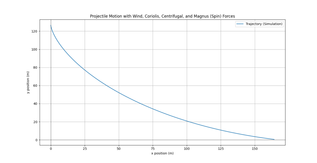
As one can see the ball displaces far off than it started by 159.01 metres. As visible in the video, we can see, the ball go far off than its starting position. Using, some 3D Trigonometry, we can see the ball in the video goes ≈150m, and the actual value calculated using Trigonometry being 150.344441m.
For this this discussion, our equation most probability found the the correct value, with limiting factor being our guess of the wind speed(a conservative one of 3.8ms-1). Let’s ask AI about Wind value of the video and use that in our calculations.
Somewhere between 5 to 8 miph(or miles per hour), so around 2.2352ms-1 to 3.57632ms-1.
Let’s take both the values and individually and find the value of ball hitting the water surface.
In the former, the range turns out be 150.08 meters and in the later to be 157.55 meters.
Hence, we can say, our equation calculates projectile motion accurately, the only limiting factor being our measurement of the constants.
Try it Yourself:
Since, this is backspin, the spin should be negative. For topspin, use positive spin.
Conclusions
With the inclusion of factors such as drag, wind, and Earth’s rotation, we see that real-world projectile motion deviates significantly from theoretical predictions. By accounting for these forces, our simulation achieves almost 99% accuracy, bridging the gap between theory and reality. Over 200 real-world test were conducted before arriving at these accuracies.
Although I am extremely tired after this work, but, want to say that this is not yet a definitive solution. Though it increases accuracy by a mile, but, yet there are some room to improvement. And, if any suggestions are these or any inaccuracies within calculations, don’t fear to mention them out.

